Particle-guided diffusion models for partial differential equations

WASP-WISE seminar: machine learning meets materials science

Zheng Zhao (w. Andrew Millard, Henrik Pedersen, Fredrik Lindsten)

Division of Statistics and Machine Learning, Linköping University

26.10.2026

Background

Continue from Henrik: computational fluid dynamics (CFD) is a key part of understanding CVD.

CFD means solving partial differential equations (PDEs), for example

• transport of species: advection, reaction and diffusion,
• flow of the carrier gas: Navier–Stokes.

The machine learning problem in this talk: solve PDEs.

What we want from a method:

1. computationally fast, at least at the time of use,
2. calibrated uncertainty quantification (UQ).

Four sources of information

Any PDE solver uses some of the following.

1. The PDE itself: the equation \(f(a, u) = 0\) and its boundary conditions.
2. Data: past simulations (e.g., CFD runs) and their results.
3. Observations: sparse measurements of the coefficient \(a\) or the solution \(u\).
4. Prior knowledge of the solution: smoothness, positivity, conservation.

Peer approaches

Approach	Data	PDE	Observations	Solution prior	Training	Fast at use	UQ
Finite difference, finite element		\(\checkmark\)			no	no	none
Probabilistic numerics		\(\checkmark\)	\(\checkmark\)	\(\checkmark\)	no	no	calibrated
PINNs, neural operators	\(\checkmark\)	\(\checkmark\)	\(\checkmark\)		yes	yes	none
Generative diffusion models	\(\checkmark\)		\(\checkmark\)		yes	yes	yes, uncalibrated
This talk	\(\checkmark\)	\(\checkmark\)	\(\checkmark\)		yes	yes	calibrated

The idea: a diffusion model trained on data, incorporating with the PDE and the observations as a likelihood, sampled with sequential Monte Carlo (SMC) for a statistical guarantee.

Probabilistic numerics gives calibrated uncertainty but is slow. PINNs and neural operators are fast but give point estimates. Diffusion models are fast and give samples, but the samples do not use the PDE and come with no guarantee.

Problem formulation

Vorticity \(\omega(c, \tau)\) of a 2D flow, physical time \(\tau\).

A PDE on a domain \(\Omega\), coordinate \(c \in \Omega\), physical time \(\tau \in [0, \calT]\): \[ \begin{aligned} f(a, u) &= 0, && c \in \Omega, \; \tau \in [0, \calT], \\ u(c, \tau) &= g(c, \tau), && c \in \partial\Omega, \\ u(c, 0) &= a(c), && c \in \Omega, \end{aligned} \] with coefficient or initial field \(a\) and solution field \(u\).

Darcy flow: \(a\) permeability, \(u\) pressure, \(-\grad \cdot (a \grad u) = s\). Navier–Stokes: \(a = \omega(\cdot, 0)\), \(u = \omega(\cdot, \tau)\) for \(\tau > 0\).

Problem formulation

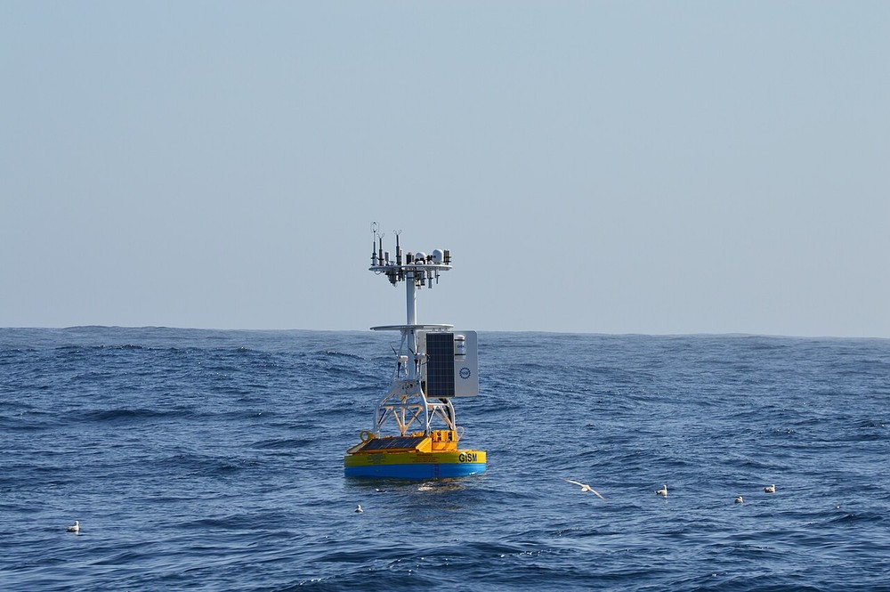
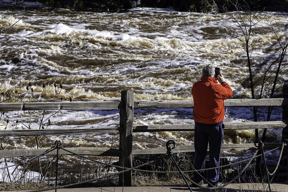
The unknown is one snapshot \(x = (a, u)\) or several.

Sparse observations \(a_\obs\) and \(u_\obs\) (black pixels).

Photos: Ocean Observatories Initiative (public domain); Lorie Shaull, CC BY 2.0, via Wikimedia Commons.

Generative diffusion models

Let \(x = (a, u) \sim \pi\), where \(\pi\) is the distribution of coefficient-solution. We have samples of \(\pi\): past CFD simulations.

Noising: run an SDE that noises the sample, for pseudo-time \(t \in [0, T]\), \[ \diff X_t = \mu_t(X_t) \diff t + \sqrt{2} \, b_t \diff W_t, \qquad X_0 \sim \pi, \qquad X_T \approx \pi_{\mathrm{ref}} = \calN(0, I). \]

Denoising: run the time reversal (Anderson, 1982), from \(Z_0 \sim \pi_{\mathrm{ref}}\), \[ \diff Z_t = \bigl[-\mu_{T-t}(Z_t) + 2 \, b_{T-t}^2 \, \alert{\grad \log p_{T-t}(Z_t)}\bigr] \diff t + \sqrt{2} \, b_{T-t} \diff W_t, \qquad Z_T \sim \pi. \]

The score \(\grad \log p_t\) is learnt from the simulations by a neural network \(s_\theta(x, t) \approx \grad\log p_t(x)\).

Diffusion models for PDE fields: Yang & Sommer (2023), Huang et al. (2024).

mu_t is a simple drift, for instance -beta_t x / 2; b_t a noise schedule. The score is the gradient of the log density of the noised data. Training only needs samples from pi, so the training set is just the archive of simulations.

Sampling a PDE solution from noise

This is no different from sampling a cat image. The sampler is purely data-driven.

Loosely speaking, this is doing fluid prediction, not solving PDE.

Cat photo: scikit-image “chelsea”, CC0.

Conditional diffusion model

Bring in the PDE and the observations through a likelihood, \(\pi(x \cond y) \propto p(y \cond x) \, \pi(x)\), with \[ \log p(y \cond x) = \underbrace{-\frac{\beta}{n} \norm{u_\obs - M_u \, u}^2 - \frac{\gamma}{n} \norm{a_\obs - M_a \, a}^2}_{\text{observations, masks } M_a, M_u} \; \underbrace{- \frac{\omega}{m} \norm{f(a, u)}^2}_{\text{PDE residual on the grid}} + \mathrm{const}. \]

The posterior is again the end point of a denoising SDE, with an extra drift term: \[ \diff Z_t = \bigl[-\mu_{T-t}(Z_t) + 2 \, b_{T-t}^2 \, \bigl(\grad \log p_{T-t}(Z_t) + \alert{\grad \log p_{T-t}(y \cond Z_t)}\bigr)\bigr] \diff t + \sqrt{2} \, b_{T-t} \diff W_t, \]

where the guidance \[ p_t(y \cond z) = \int p(y \cond x) \, p(x \cond X_t = z) \diff x \;\approx\; p\bigl(y \cond D_\theta(z, t)\bigr), \qquad D_\theta(z, t) \approx \expec{X_0 \cond X_t = z}, \] with the trained denoiser \(D_\theta\).

Guided sampling

At each \(t\): predict, evaluate the likelihood, then move along the gradient (Huang et al., 2024).

Guided sampling is biased

The guided SDE does not sample \(\pi(x \cond y)\). Three sources of error:

1. The intermediate likelihood \(p_t(y \cond z)\) is \(\approx\) by a point estimate \(p(y \cond D_\theta(z, t))\).

2. The SDE is time-discretised.

3. The learned prior \(\pi_\theta\) is not the actual \(\pi\).

Fix: keep the guided trajectory as a proposal, and correct it with sequential Monte Carlo.

Sequential Monte Carlo

Discretise the pseudo-time, \(t_K = 0 < \cdots < t_k < \cdots < t_0 = T\), and run \(N\) guided trajectories (particles) in parallel. For \(k = K, \ldots, 1\) and each particle \(i = 1, \ldots, N\):

1. Propose: \(Z_{k-1}^{(i)} \sim M_{k-1}\bigl(\cdot \cond Z_k^{(i)}\bigr)\), one step of the guided SDE.
2. Weight: \(w_{k-1}^{(i)} \propto w_k^{(i)} \, G_{k-1}\bigl(Z_k^{(i)}, Z_{k-1}^{(i)}\bigr)\).
3. Resample

The weighted particles target a sequence of distributions (Feynman–Kac), \[ \nu_k(z_{k:K}) \propto G_K(z_K) \, M_K(z_K) \prod_{j=k+1}^{K} G_{j-1}(z_j, z_{j-1}) \, M_{j-1}(z_{j-1} \cond z_j). \]

Choose \(M\) and \(G\) so that the last marginal is the posterior, \(\nu_0(z_0) = \pi_\theta(z_0 \cond y)\). Then \(\sum_{i=1}^N w^{(i)} \phi\bigl(Z_0^{(i)}\bigr) \to \expec{\phi(x) \cond y}\) as \(N \to \infty\): a statistical guarantee.

Particles, weights and resampling

From diffusion to PINNs

The framework allows for a more flexible family of targets: \[ \overline{\nu}_\rho(x) \propto \overline{p}_\theta(x \cond y) \, p(y \cond x)^{\rho}, \]

• \(\rho = 0\): plain guided sampling (DiffusionPDE), the data prior dominates.
• \(\rho = 1\): an instance of our particle system.
• \(\rho \to \infty\): the likelihood becomes sharp, fitting the PDE residual and observations: a PINN.

The tempering parameter is also the knob that controls calibration of the uncertainty: with rho = 1 the spread of the particles is a Bayesian posterior spread for the chosen target.

Benefits

• Calibrated UQ: weighted particles are a consistent Monte Carlo estimate of the target posterior.
• Fast at inference: Training is the most notorious, but after training, everything is fast.
• The PDE is used: through the likelihood in the guidance.
• One tuning parameter \(\rho\) that interpolates between a data-driven sampler and a PINN.

Approach	Data	PDE	Observations	Training	Fast at use	UQ
Generative diffusion models	\(\checkmark\)		\(\checkmark\)	yes	yes	uncalibrated
Particle-guided diffusion	\(\checkmark\)	\(\checkmark\)	\(\checkmark\)	yes	yes	calibrated

Benchmarks

Five PDEs, pretrained DiffusionPDE priors, \(128 \times 128\) fields, 3% of pixels observed, \(N = 4\) particles.

Relative \(L_2\) error (%)	Darcy		Poisson		Helmholtz		Navier–Stokes		NS with BCs
	fwd	inv	fwd	inv	fwd	inv	fwd	inv	fwd	inv
DiffusionPDE (ODE guidance)	5.58	8.31	8.67	19.88	17.49	19.14	4.27	9.34	2.78	3.43
Ours, GEM-pBS, \(N = 4\)	4.49	5.74	8.73	22.01	9.01	18.89	4.27	10.12	2.01	2.32
Ours, SOSaG-pBS, \(N = 4\)	3.96	5.28	8.68	24.61	12.99	20.50	4.22	11.24	2.08	2.17

fwd: observe \(a\), recover \(u\); inv: observe \(u\), recover \(a\). Navier–Stokes: \(a\) initial state, \(u\) end state. Darcy inv: error rate.

Application: gas-phase reaction kinetics

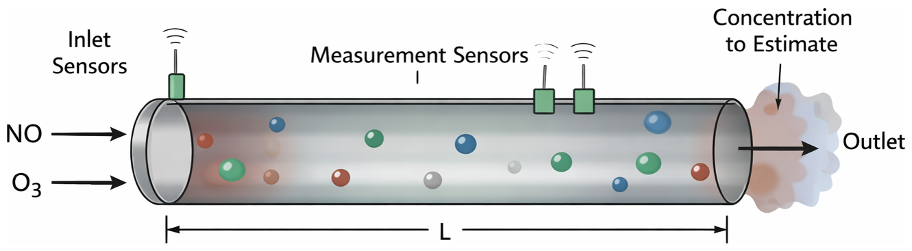
Concentrations \(C_s(c, \tau)\) of species \(s\) at \(c = (r, z)\) in a tube reactor, laminar flow \(v(r) = 2\,\bar{v}\,(1 - r^2/A^2)\): \[ \tash{C_s}{\tau} + v(r)\,\tash{C_s}{z} = D_s \Bigl( \tash{^2 C_s}{z^2} + \frac{1}{r}\tash{}{r}\Bigl( r\,\tash{C_s}{r} \Bigr) \Bigr) + R_s(C). \]

Millard, Zhao & Pedersen, ProbNum 2026; Millard & Pedersen, AI&PDE @ ICLR 2026

Reconstruction in physical time

NO + O₃ → NO₂ + O₂. Empirical prior of 1,000 simulations at random \(T\), \(\bar v\), \(D\) and inlet feed. SMC with \(N = 24\) particles at each \(\tau_n\).

More species: methanol–formaldehyde network

CH₂O + H₂ ⇌ CH₃OH, CH₂O → CO + H₂, CH₃OH + CO → HCOOCH₃

More species: NO_x network

NO + O₃ → NO₂ + O₂, 2 NO₂ ⇌ N₂O₄, NO + NO₂ ⇌ N₂O₃. \(N = 32\) particles, weights tempered with \(\rho = 0.7\).

Summary

• Solving a PDE with a diffusion model trained on data.
• Incorporating physical and observation guidance.
• Giving calibrated uncertainty.
• A tempering parameter \(\rho\) connects the method to PINNs.
• It works on benchmark PDEs and on gas-phase reaction kinetics in a simple CVD reactor.

Thank you!
waspwise2025.spdes.net